
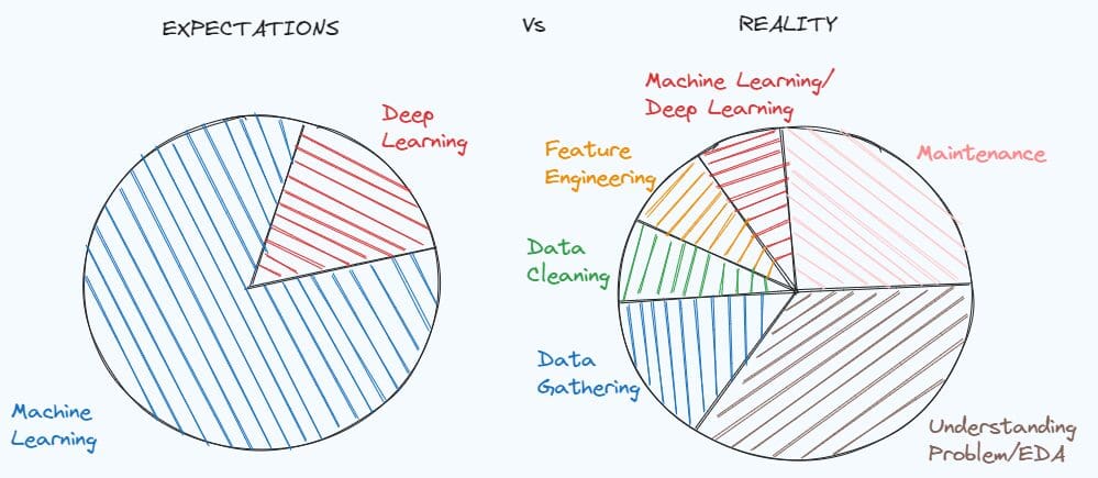
Illustration by Writer. Impressed by MEME of Dr. Angshuman Ghosh
Mastering Knowledge Cleansing and Preprocessing Methods is basic for fixing quite a lot of information science initiatives. A easy demonstration of how essential could be discovered within the meme concerning the expectations of a pupil finding out information science earlier than working, in contrast with the truth of the info scientist job.
We are likely to idealise the job place earlier than having a concrete expertise, however the actuality is that it’s all the time totally different from what we actually count on. When working with a real-world drawback, there isn’t a documentation of the info and the dataset could be very soiled. First, you must dig deep in the issue, perceive what clues you’re lacking and what info you possibly can extract.
After understanding the issue, that you must put together the dataset in your machine studying mannequin for the reason that information in its preliminary situation is rarely sufficient. On this article, I’m going to indicate seven steps that may enable you to on pre-processing and cleansing your dataset.
Step one in a knowledge science venture is the exploratory evaluation, that helps in understanding the issue and taking choices within the subsequent steps. It tends to be skipped, nevertheless it’s the worst error since you’ll lose quite a lot of time later to search out the explanation why the mannequin provides errors or didn’t carry out as anticipated.
Based mostly on my expertise as information scientist, I’d divide the exploratory evaluation into three elements:
- Verify the construction of the dataset, the statistics, the lacking values, the duplicates, the distinctive values of the explicit variables
- Perceive the which means and the distribution of the variables
- Examine the relationships between variables
To analyse how the dataset is organised, there are the next Pandas strategies that may enable you to:
df.head()
df.information()
df.isnull().sum()
df.duplicated().sum()
df.describe([x*0.1 for x in range(10)])
 for c in record(df):
    print(df[c].value_counts())
When attempting to know the variables, it’s helpful to separate the evaluation into two additional elements: numerical options and categorical options. First, we will give attention to the numerical options that may be visualised via histograms and boxplots. After, it’s the flip for the explicit variables. In case it’s a binary drawback, it’s higher to begin by trying if the courses are balanced. After our consideration could be centered on the remaining categorical variables utilizing the bar plots. In the long run, we will lastly test the correlation between every pair of numerical variables. Different helpful information visualisations could be the scatter plots and boxplots to watch the relations between a numerical and a categorical variable.
In step one, we’ve already investigated if there are missings in every variable. In case there are lacking values, we have to perceive deal with the difficulty. The best method can be to take away the variables or the rows that comprise NaN values, however we would like to keep away from it as a result of we danger dropping helpful info that may assist our machine studying mannequin on fixing the issue.
If we’re coping with a numerical variable, there are a number of approaches to fill it. The preferred technique consists in filling the lacking values with the imply/median of that characteristic:
df['age'].fillna(df['age'].imply())
df['age'].fillna(df['age'].median())
One other method is to substitute the blanks with group by imputations:
df['price'].fillna(df.group('type_building')['price'].rework('imply'),
inplace=True)
It may be a greater possibility in case there’s a robust relationship between a numerical characteristic and a categorical characteristic.
In the identical method, we will fill the lacking values of categorical based mostly on the mode of that variable:
df['type_building'].fillna(df['type_building'].mode()[0])
If there are duplicates throughout the dataset, it’s higher to delete the duplicated rows:
df = df.drop_duplicates()
Whereas deciding deal with duplicates is straightforward, coping with outliers could be difficult. That you must ask your self “Drop or not Drop Outliers?”.
Outliers ought to be deleted in case you are positive that they supply solely noisy info. For instance, the dataset incorporates two individuals with 200 years, whereas the vary of the age is between 0 and 90. In that case, it’s higher to take away these two information factors.
Sadly, more often than not eradicating outliers can result in dropping essential info. Probably the most environment friendly method is to use the logarithm transformation to the numerical characteristic.
One other approach that I found throughout my final expertise is the clipping technique. On this approach, you select the higher and the decrease certain, that may be the 0.1 percentile and the 0.9 percentile. The values of the characteristic beneath the decrease certain will probably be substituted with the decrease certain worth, whereas the values of the variable above the higher certain will probably be changed with the higher certain worth.
for c in columns_with_outliers:
   rework= 'clipped_'+ c
   lower_limit = df[c].quantile(0.10)
   upper_limit = df[c].quantile(0.90)
   df[transform] = df[c].clip(lower_limit, upper_limit, axis = 0)
The following section is to transform the explicit options into numerical options. Certainly, the machine studying mannequin is in a position solely to work with numbers, not strings.
Earlier than going additional, it’s best to distinguish between two kinds of categorical variables: non-ordinal variables and ordinal variables.
Examples of non-ordinal variables are the gender, the marital standing, the kind of job. So, it’s non-ordinal if the variable doesn’t observe an order, otherwise from the ordinal options. An instance of ordinal variables could be the schooling with values “childhood”, “main”, “secondary” and “tertiary”, and the revenue with ranges “low”, “medium” and “excessive”.
Once we are coping with non-ordinal variables, One-Sizzling Encoding is the most well-liked approach taken under consideration to transform these variables into numerical.
On this technique, we create a brand new binary variable for every stage of the explicit characteristic. The worth of every binary variable is 1 when the identify of the extent coincides with the worth of the extent, 0 in any other case.
from sklearn.preprocessing import OneHotEncoder

data_to_encode = df[cols_to_encode]
encoder = OneHotEncoder(dtype="int")
encoded_data = encoder.fit_transform(data_to_encode)
dummy_variables = encoder.get_feature_names_out(cols_to_encode)
encoded_df = pd.DataFrame(encoded_data.toarray(), columns=encoder.get_feature_names_out(cols_to_encode))

final_df = pd.concat([df.drop(cols_to_encode, axis=1), encoded_df], axis=1)
When the variable is ordinal, the most typical approach used is the Ordinal Encoding, which consists in changing the distinctive values of the explicit variable into integers that observe an order. For instance, the degrees “low”, “Medium” and “Excessive” of revenue will probably be encoded respectively as 0,1 and a couple of.
from sklearn.preprocessing import OrdinalEncoder

data_to_encode = df[cols_to_encode]
encoder = OrdinalEncoder(dtype="int")
encoded_data = encoder.fit_transform(data_to_encode)
encoded_df = pd.DataFrame(encoded_data.toarray(), columns=["Income"])

final_df = pd.concat([df.drop(cols_to_encode, axis=1), encoded_df], axis=1)
There are different attainable encoding methods if you wish to discover right here. You may have a look right here in case you have an interest in alternate options.
It’s time to divide the dataset into three fastened subsets: the most typical alternative is to make use of 60% for coaching, 20% for validation and 20% for testing. As the amount of knowledge grows, the share for coaching will increase and the share for validation and testing decreases.
It’s essential to have three subsets as a result of the coaching set is used to coach the mannequin, whereas the validation and the check units could be helpful to know how the mannequin is acting on new information.
To separate the dataset, we will use the train_test_split of scikit-learn:
from sklearn.model_selection import train_test_split

X = final_df.drop(['y'],axis=1)
y = final_df['y']

train_idx, test_idx,_,_ = train_test_split(X.index,y,test_size=0.2,random_state=123)
train_idx, val_idx,_,_ = train_test_split(train_idx,y_train,test_size=0.2,random_state=123)

df_train = final_df[final_df.index.isin(train_idx)]
df_test = final_df[final_df.index.isin(test_idx)]
df_val = final_df[final_df.index.isin(val_idx)]
In case we’re coping with a classification drawback and the courses are usually not balanced, it’s higher to arrange the stratify argument to ensure that there is identical proportion of courses in coaching, validation and check units.
train_idx, test_idx,y_train,_ = train_test_split(X.index,y,test_size=0.2,stratify=y,random_state=123)
train_idx, val_idx,_,_ = train_test_split(train_idx,y_train,test_size=0.2,stratify=y_train,random_state=123)
This stratified cross-validation additionally helps to make sure that there is identical proportion of the goal variable within the three subsets and provides extra correct performances of the mannequin.
There are machine studying fashions, like Linear Regression, Logistic Regression, KNN, Help Vector Machine and Neural Networks, that require scaling options. The characteristic scaling solely helps the variables be in the identical vary, with out altering the distribution.
There are three hottest characteristic scaling methods are Normalization, Standardization and Sturdy scaling.
Normalization, aso referred to as min-max scaling, consists of mapping the worth of a variable into a spread between 0 and 1. That is attainable by subtracting the minimal of the characteristic from the characteristic worth and, then, dividing by the distinction between the utmost and the minimal of that characteristic.
from sklearn.preprocessing import MinMaxScaler
sc=MinMaxScaler()
df_train[numeric_features]=sc.fit_transform(df_train[numeric_features])
df_test[numeric_features]=sc.rework(df_test[numeric_features])
df_val[numeric_features]=sc.rework(df_val[numeric_features])
One other frequent method is Standardization, that rescales the values of a column to respect the properties of a typical regular distribution, which is characterised by imply equal to 0 and variance equal to 1.
from sklearn.preprocessing import StandardScaler
sc=StandardScaler()
df_train[numeric_features]=sc.fit_transform(df_train[numeric_features])
df_test[numeric_features]=sc.rework(df_test[numeric_features])
df_val[numeric_features]=sc.rework(df_val[numeric_features])
If the characteristic incorporates outliers that can’t be eliminated, a preferable technique is the Sturdy Scaling, that rescales the values of a characteristic based mostly on strong statistics, the median, the primary and the third quartile. The rescaled worth is obtained by subtracting the median from the unique worth and, then, dividing by the Interquartile Vary, which is the distinction between the seventy fifth and twenty fifth quartile of the characteristic.
from sklearn.preprocessing import RobustScaler
sc=RobustScaler()
df_train[numeric_features]=sc.fit_transform(df_train[numeric_features])
df_test[numeric_features]=sc.rework(df_test[numeric_features])
df_val[numeric_features]=sc.rework(df_val[numeric_features])
Typically, it’s preferable to calculate the statistics based mostly on the coaching set after which use them to rescale the values on each coaching, validation and check units. It’s because we suppose that we solely have the coaching information and, later, we wish to check our mannequin on new information, which ought to have an analogous distribution than the coaching set.
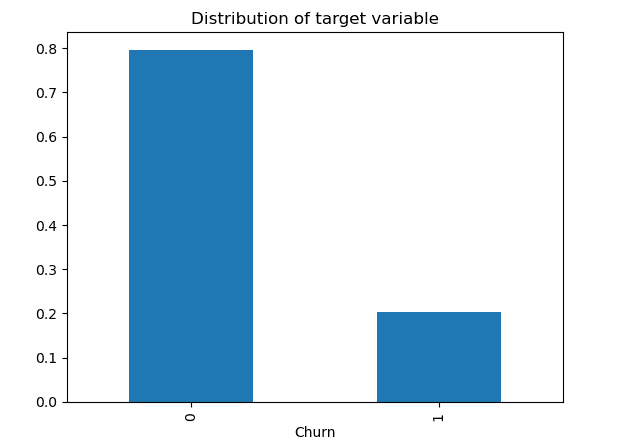
This step is simply included once we are working in a classification drawback and we’ve discovered that the courses are imbalanced.
In case there’s a slight distinction between the courses, for instance class 1 incorporates 40% of the observations and sophistication 2 incorporates the remaining 60%, we don’t want to use oversampling or undersampling methods to change the variety of samples in one of many courses. We are able to simply keep away from taking a look at accuracy because it’s a superb measure solely when the dataset is balanced and we must always care solely about analysis measures, like precision, recall and f1-score.
However it could possibly occur that the constructive class has a really low proportion of knowledge factors (0.2) in comparison with the detrimental class (0.8). The machine studying might not carry out effectively with the category with much less observations, resulting in failing on fixing the duty.
To beat this problem, there are two prospects: undersampling the bulk class and oversampling the minority class. Undersampling consists in lowering the variety of samples by randomly eradicating some information factors from the bulk class, whereas Oversampling will increase the variety of observations within the minority class by including randomly information factors from the much less frequent class. There’s the imblearn that enables to steadiness the dataset with few strains of code:
# undersampling
from imblearn.over_sampling import RandomUnderSampler,RandomOverSampler
undersample = RandomUnderSampler(sampling_strategy='majority')
X_train, y_train = undersample.fit_resample(df_train.drop(['y'],axis=1),df_train['y'])
# oversampling
oversample = RandomOverSampler(sampling_strategy='minority')
X_train, y_train = oversample.fit_resample(df_train.drop(['y'],axis=1),df_train['y'])
Nonetheless, eradicating or duplicating among the observations could be ineffective generally in bettering the efficiency of the mannequin. It could be higher to create new synthetic information factors within the minority class. A way proposed to unravel this problem is SMOTE, which is understood for producing artificial data within the class much less represented. Like KNN, the thought is to determine okay nearest neighbors of observations belonging to the minority class, based mostly on a specific distance, like t. After a brand new level is generated at a random location between these okay nearest neighbors. This course of will hold creating new factors till the dataset is totally balanced.
from imblearn.over_sampling import SMOTE
resampler = SMOTE(random_state=123)
X_train, y_train = resampler.fit_resample(df_train.drop(['y'],axis=1),df_train['y'])
I ought to spotlight that these approaches ought to be utilized solely to resample the coaching set. We would like that our machine mannequin learns in a strong method and, then, we will apply it to make predictions on new information.
I hope you might have discovered this complete tutorial helpful. It may be arduous to begin our first information science venture with out being conscious of all these methods. You could find all my code right here.
There are certainly different strategies I didn’t cowl within the article, however I most well-liked to give attention to the most well-liked and recognized ones. Do you might have different strategies? Drop them within the feedback when you’ve got insightful strategies.
Helpful sources:
Eugenia Anello is at the moment a analysis fellow on the Division of Data Engineering of the College of Padova, Italy. Her analysis venture is concentrated on Continuous Studying mixed with Anomaly Detection.