

Picture by Creator
Linear Regression is among the most basic instruments in machine studying. It’s used to discover a straight line that matches our information effectively. Though it solely works with easy straight-line patterns, understanding the mathematics behind it helps us perceive Gradient Descent and Loss Minimization strategies. These are essential for extra difficult fashions utilized in all machine studying and deep studying duties.
On this article, we’ll roll up our sleeves and construct Linear Regression from scratch utilizing NumPy. As an alternative of utilizing summary implementations similar to these supplied by Scikit-Be taught, we are going to begin from the fundamentals.
We generate a dummy dataset utilizing Scikit-Be taught strategies. We solely use a single variable for now, however the implementation will likely be common that may prepare on any variety of options.
The make_regression technique supplied by Scikit-Be taught generates random linear regression datasets, with added Gaussian noise so as to add some randomness.
X, y = datasets.make_regression(
        n_samples=500, n_features=1, noise=15, random_state=4)
We generate 500 random values, every with 1 single function. Subsequently, X has form (500, 1) and every of the five hundred impartial X values, has a corresponding y worth. So, y additionally has form (500, ).
Visualized, the dataset seems to be as follows:
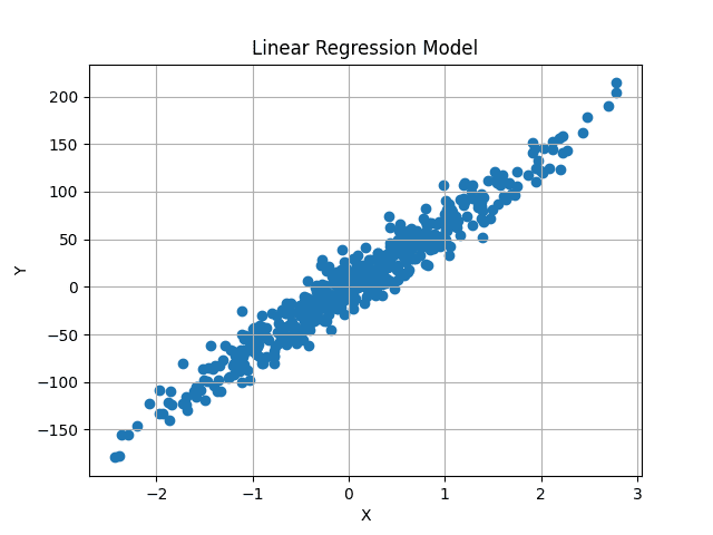
Picture by Creator
We purpose to discover a best-fit line that passes via the middle of this information, minimizing the common distinction between the anticipated and unique y values.
The overall equation for a linear line is:
y = m*X + b
X is numeric, single-valued. Right here m and b characterize the gradient and y-intercept (or bias). These are unknowns, and ranging values of those can generate totally different traces. In machine studying, X depends on the info, and so are the y values. We solely have management over m and b, that act as our mannequin parameters. We purpose to seek out optimum values of those two parameters, that generate a line that minimizes the distinction between predicted and precise y values.
This extends to the state of affairs the place X is multi-dimensional. In that case, the variety of m values will equal the variety of dimensions in our information. For instance, if our information has three totally different options, we could have three totally different m values, known as weights.
The equation will now turn out to be:
y = w1*X1 + w2*X2 + w3*X3 + b
This will then lengthen to any variety of options.
However how do we all know the optimum values of our bias and weight values? Nicely, we don’t. However we are able to iteratively discover it out utilizing Gradient Descent. We begin with random values and alter them barely for a number of steps till we get near the optimum values.
First, allow us to initialize Linear Regression, and we are going to go over the optimization course of in larger element later.
import numpy as np


class LinearRegression:
    def __init__(self, lr: int = 0.01, n_iters: int = 1000) -> None:
        self.lr = lr
        self.n_iters = n_iters
        self.weights = None
        self.bias = None
We use a studying charge and variety of iterations hyperparameters, that will likely be defined later. The weights and biases are set to None as a result of the variety of weight parameters depends upon the enter options throughout the information. We shouldn’t have entry to the info but, so we initialize them to None for now.
Within the match technique, we’re supplied with information and their related values. We are able to now use these, to initialize our weights, after which prepare the mannequin to seek out optimum weights.
def match(self, X, y):
        num_samples, num_features = X.form     # X form [N, f]
        self.weights = np.random.rand(num_features)  # W form [f, 1]
        self.bias = 0
The impartial function X will likely be a NumPy array of form (num_samples, num_features). In our case, the form of X is (500, 1). Every row in our information could have an related goal worth, so y can also be of form (500,) or (num_samples).
We extract this and randomly initialize the weights given the variety of enter options. So now our weights are additionally a NumPy array of dimension (num_features, ). Bias is a single worth initialized to zero.
We use the road equation mentioned above to calculate predicted y values. Nevertheless, as a substitute of an iterative strategy to sum all values, we are able to comply with a vectorized strategy for sooner computation. Provided that the weights and X values are NumPy arrays, we are able to use matrix multiplication to get predictions.
X has form (num_samples, num_features) and weights have form (num_features, ). We wish the predictions to be of form (num_samples, ) matching the unique y values. Subsequently we are able to multiply X with weights, or (num_samples, num_features) x (num_features, ) to acquire predictions of form (num_samples, ).
The bias worth is added on the finish of every prediction. This will merely be applied in a single line.
# y_pred form ought to be N, 1
y_pred = np.dot(X, self.weights) + self.bias
Nevertheless, are these predictions right? Clearly not. We’re utilizing randomly initialized values for the weights and bias, so the predictions may even be random.
How will we get the optimum values? Gradient Descent.
Now that now we have each predicted and goal y values, we are able to discover the distinction between each values. Imply Sq. Error (MSE) is used to check real-valued numbers. The equation is as follows:
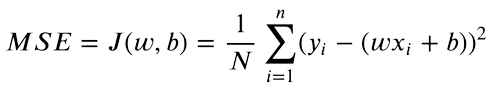
We solely care in regards to the absolute distinction between our values. A prediction larger than the unique worth is as dangerous as a decrease prediction. So we sq. the distinction between our goal worth and predictions, to transform adverse variations to constructive. Furthermore, this penalizes a bigger distinction between targets and predictions, as larger variations squared will contribute extra to the ultimate loss.
For our predictions to be as near unique targets as potential, we now attempt to decrease this perform. The loss perform will likely be minimal, the place the gradient is zero. As we are able to solely optimize our weights and bias values, we take the partial derivates of the MSE perform with respect to weights and bias values.
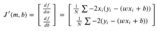
We then optimize our weights given the gradient values, utilizing Gradient Descent.
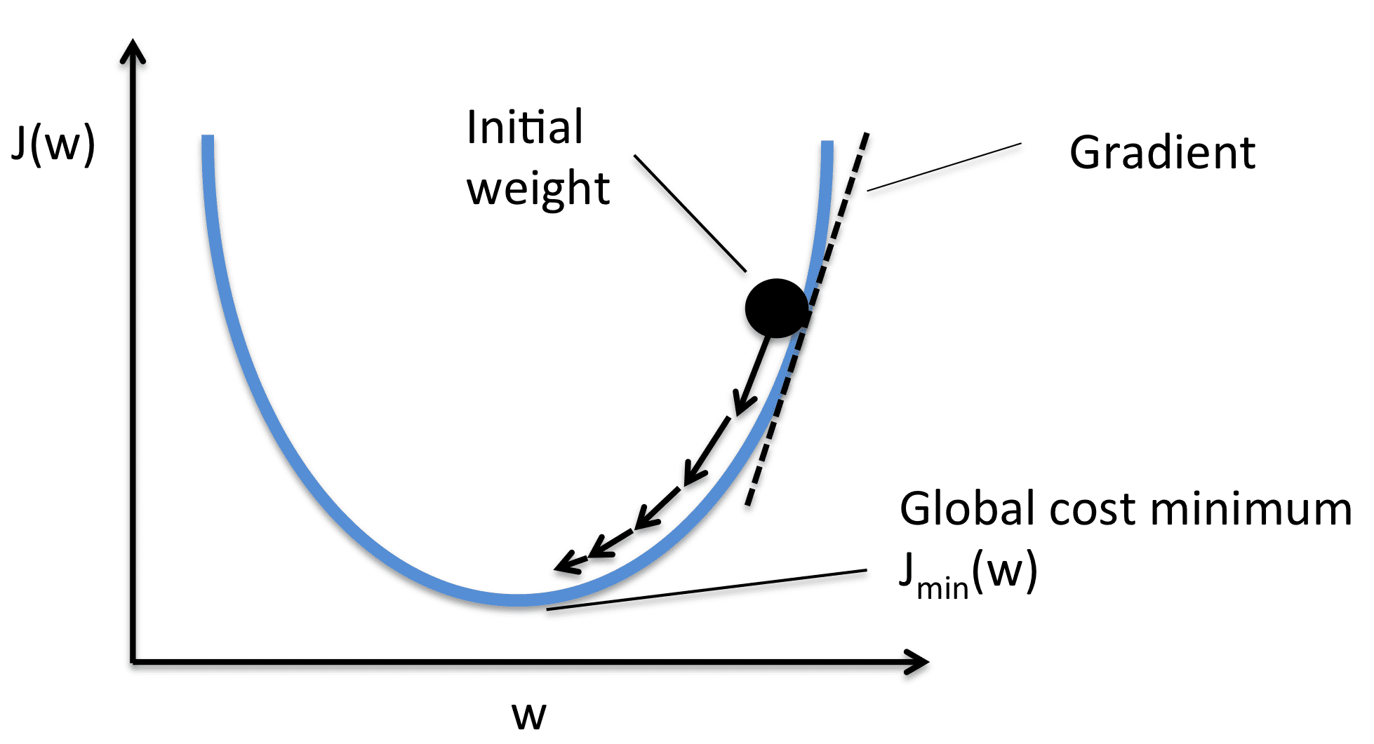
Picture from Sebasitan Raschka
We take the gradient with respect to every weight worth after which transfer them to the alternative of the gradient. This pushes the the loss in the direction of minimal. As per the picture, the gradient is constructive, so we lower the load. This pushes the J(W) or loss in the direction of the minimal worth. Subsequently, the optimization equations look as follows:
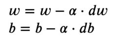
The training charge (or alpha) controls the incremental steps proven within the picture. We solely make a small change within the worth, for steady motion in the direction of the minimal.
Implementation
If we simplify the derivate equation utilizing primary algebraic manipulation, this turns into quite simple to implement.
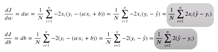
For the derivate, we implement this utilizing two traces of code:
# X -> [ N, f ]
# y_pred -> [ N ]
# dw -> [ f ]
dw = (1 / num_samples) * np.dot(X.T, y_pred - y)
db = (1 / num_samples) * np.sum(y_pred - y)
dw is once more of form (num_features, ) So now we have a separate derivate worth for every weight. We optimize them individually. db has a single worth.
To optimize the values now, we transfer the values in the other way of the gradient utilizing primary subtraction.
self.weights = self.weights - self.lr * dw
self.bias = self.bias - self.lr * db
Once more, that is solely a single step. We solely make a small change to the randomly initialized values. We now repeatedly carry out the identical steps, to converge in the direction of a minimal.
The whole loop is as follows:
for i in vary(self.n_iters):

            # y_pred form ought to be N, 1
            y_pred = np.dot(X, self.weights) + self.bias

            # X -> [N,f]
            # y_pred -> [N]
            # dw -> [f]
            dw = (1 / num_samples) * np.dot(X.T, y_pred - y)
            db = (1 / num_samples) * np.sum(y_pred - y)

            self.weights = self.weights - self.lr * dw
            self.bias = self.bias - self.lr * db
We predict the identical approach as we did throughout coaching. Nevertheless, now now we have the optimum set of weights and biases. The expected values ought to now be near the unique values.
def predict(self, X):
        return np.dot(X, self.weights) + self.bias
With randomly initialized weights and bias, our predictions had been as follows:
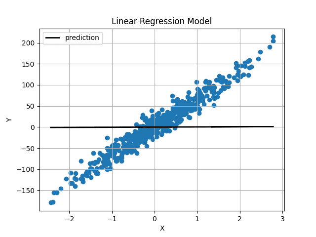
Picture by Creator
Weight and bias had been initialized very near 0, so we acquire a horizontal line. After coaching the mannequin for 1000 iterations, we get this:
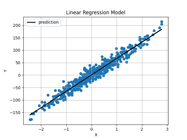
Picture by Creator
The expected line passes proper via the middle of our information and appears to be the best-fit line potential.
You’ve got now applied Linear Regression from scratch. The whole code can also be out there on GitHub.
import numpy as np


class LinearRegression:
    def __init__(self, lr: int = 0.01, n_iters: int = 1000) -> None:
        self.lr = lr
        self.n_iters = n_iters
        self.weights = None
        self.bias = None

    def match(self, X, y):
        num_samples, num_features = X.form     # X form [N, f]
        self.weights = np.random.rand(num_features)  # W form [f, 1]
        self.bias = 0

        for i in vary(self.n_iters):

            # y_pred form ought to be N, 1
            y_pred = np.dot(X, self.weights) + self.bias

            # X -> [N,f]
            # y_pred -> [N]
            # dw -> [f]
            dw = (1 / num_samples) * np.dot(X.T, y_pred - y)
            db = (1 / num_samples) * np.sum(y_pred - y)

            self.weights = self.weights - self.lr * dw
            self.bias = self.bias - self.lr * db

        return self

    def predict(self, X):
        return np.dot(X, self.weights) + self.bias
Muhammad Arham is a Deep Studying Engineer working in Laptop Imaginative and prescient and Pure Language Processing. He has labored on the deployment and optimizations of a number of generative AI purposes that reached the worldwide prime charts at Vyro.AI. He’s keen on constructing and optimizing machine studying fashions for clever methods and believes in continuous enchancment.