
Picture by Writer
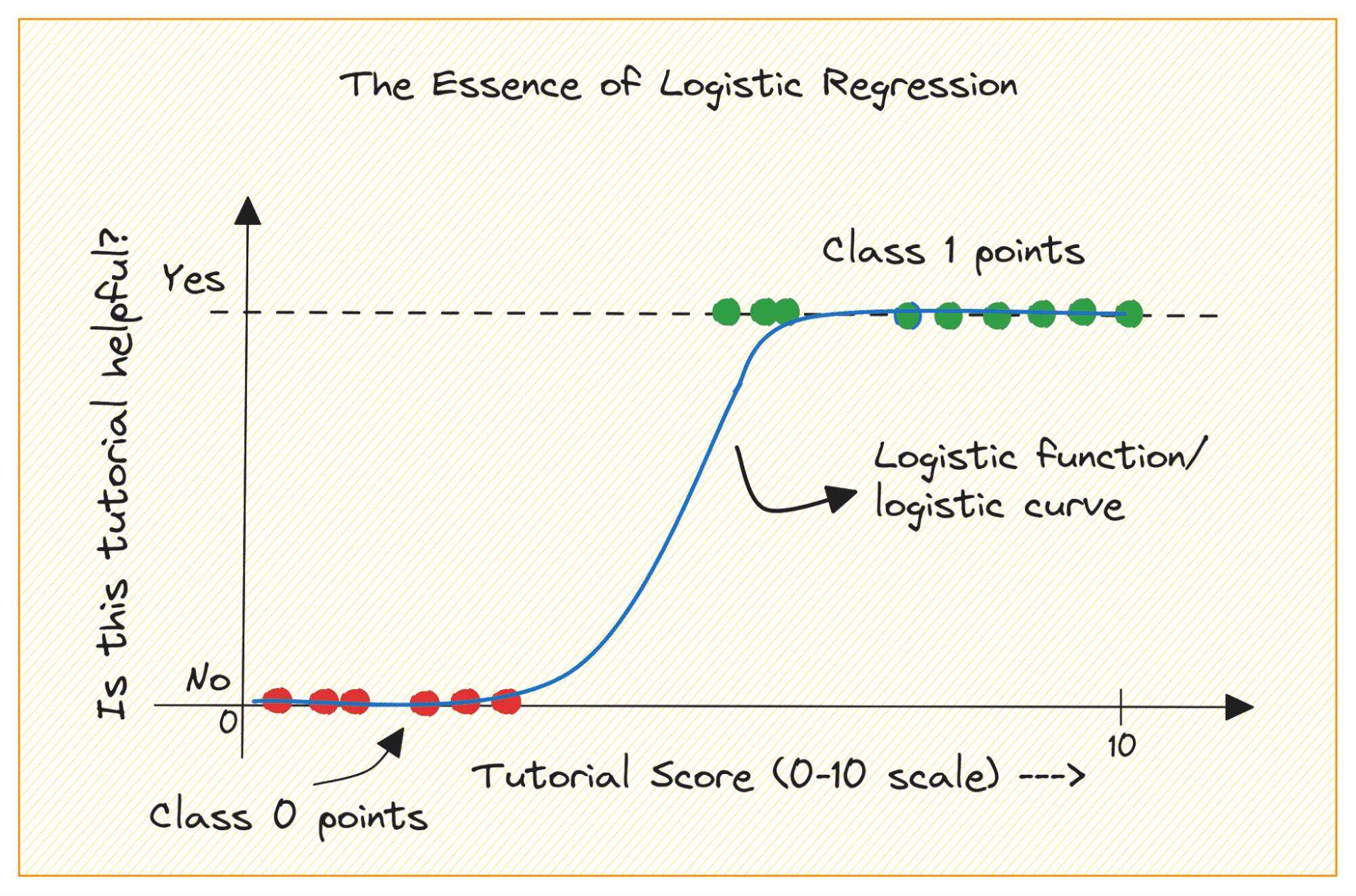
When you find yourself getting began with machine studying, logistic regression is among the first algorithms you’ll add to your toolbox. It is a easy and strong algorithm, generally used for binary classification duties.
Take into account a binary classification drawback with lessons 0 and 1. Logistic regression suits a logistic or sigmoid perform to the enter knowledge and predicts the likelihood of a question knowledge level belonging to class 1. Attention-grabbing, sure?
On this tutorial, we’ll study logistic regression from the bottom up masking:
- The logistic (or sigmoid) perform
- How we transfer from linear to logistic regression
- How logistic regression works
Lastly, we’ll construct a easy logistic regression mannequin to classify RADAR returns from the ionosphere.
Earlier than we be taught extra about logistic regression, let’s evaluation how the logistic perform works. The logistic (or sigmoid perform) is given by:

Whenever you plot the sigmoid perform, it’ll seem like so:
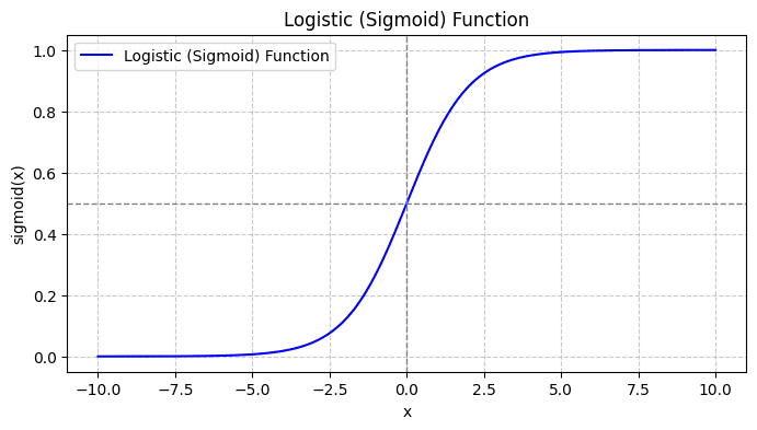
From the plot, we see that:
- When x = 0, σ(x) takes a worth of 0.5.
- When x approaches +∞, σ(x) approaches 1.
- When x approaches -∞, σ(x) approaches 0.
So for all actual inputs, the sigmoid perform squishes them to tackle values within the vary [0, 1].
Let’s first focus on why we can’t use linear regression for a binary classification drawback.
In a binary classification drawback, the output is categorical label (0 or 1). As a result of linear regression predicts continuous-valued outputs which might be lower than 0 or better than 1, it doesn’t make sense for the issue at hand.
Additionally, a straight line is probably not one of the best match when the output labels belong to one of many two classes.

Picture by Writer
So how will we go from linear to logistic regression? In linear regression the anticipated output is given by:

The place the βs are the coefficients and X_is are the predictors (or options).
With out lack of generality, let’s assume X_0 = 1:

So we will have a extra concise expression:

In logistic regression, we want the anticipated likelihood p_i within the [0,1] interval. We all know that the logistic perform squishes inputs in order that they tackle values within the [0,1] interval.
So plugging on this expression into the logistic perform, we’ve the anticipated likelihood as:

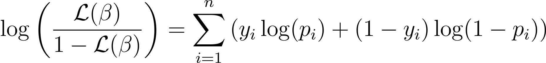
So how do we discover one of the best match logistic curve for the given knowledge set? To reply this, let’s perceive most probability estimation.
Most Chance Estimation (MLE) is used to estimate the parameters of the logistic regression mannequin by maximizing the probability perform. Let’s break down the method of MLE in logistic regression and the way the fee perform is formulated for optimization utilizing gradient descent.
Breaking Down Most Chance Estimation
As mentioned, we mannequin the likelihood {that a} binary final result happens as a perform of a number of predictor variables (or options):

Right here, the βs are the mannequin parameters or coefficients. X_1, X_2,…, X_n are the predictor variables.
MLE goals to search out the values of β that maximize the probability of the noticed knowledge. The probability perform, denoted as L(β), represents the likelihood of observing the given outcomes for the given predictor values below the logistic regression mannequin.
Formulating the Log-Chance Operate
To simplify the optimization course of, it’s normal to work with the log-likelihood perform. As a result of it transforms merchandise of chances into sums of log chances.
The log-likelihood perform for logistic regression is given by:
Now that we all know the essence of log-likelihood, let’s proceed to formulate the fee perform for logistic regression and subsequently gradient descent for locating one of the best mannequin parameters
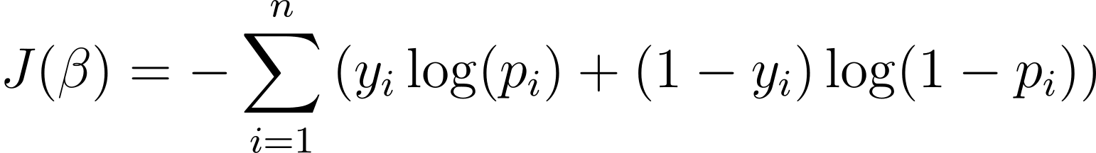
Price Operate for Logistic Regression
To optimize the logistic regression mannequin, we have to maximize the log-likelihood. So we will use the unfavorable log-likelihood as the fee perform to decrease throughout coaching. The unfavorable log-likelihood, also known as the logistic loss, is outlined as:
The objective of the training algorithm, due to this fact, is to search out the values of ? that decrease this value perform. Gradient descent is a generally used optimization algorithm for locating the minimal of this value perform.
Gradient Descent in Logistic Regression
Gradient descent is an iterative optimization algorithm that updates the mannequin parameters β in the wrong way of the gradient of the fee perform with respect to β. The replace rule at step t+1 for logistic regression utilizing gradient descent is as follows:

The place α is the training charge.
The partial derivatives might be computed utilizing the chain rule. Gradient descent iteratively updates the parameters—till convergence—aiming to reduce the logistic loss. Because it converges, it finds the optimum values of β that maximize the probability of the noticed knowledge.
Now that you understand how logistic regression works, let’s construct a predictive mannequin utilizing the scikit-learn library.
We’ll use the ionosphere dataset from the UCI machine studying repository for this tutorial. The dataset contains 34 numerical options. The output is binary, considered one of ‘good’ or ‘dangerous’ (denoted by ‘g’ or ‘b’). The output label ‘good’ refers to RADAR returns which have detected some construction within the ionosphere.
Step 1 – Loading the Dataset
First, obtain the dataset and browse it right into a pandas dataframe:
import pandas as pd
import urllib

url = "https://archive.ics.uci.edu/ml/machine-learning-databases/ionosphere/iphere.knowledge"
knowledge = urllib.request.urlopen(url)
df = pd.read_csv(knowledge, header=None)
Step 2 – Exploring the Dataset
Let’s check out the primary few rows of the dataframe:
# Show the primary few rows of the DataFrame
df.head()
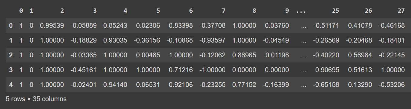
Truncated Output of df.head()
Let’s get some details about the dataset: the variety of non-null values and the information forms of every of the columns:
# Get details about the dataset
print(df.information())
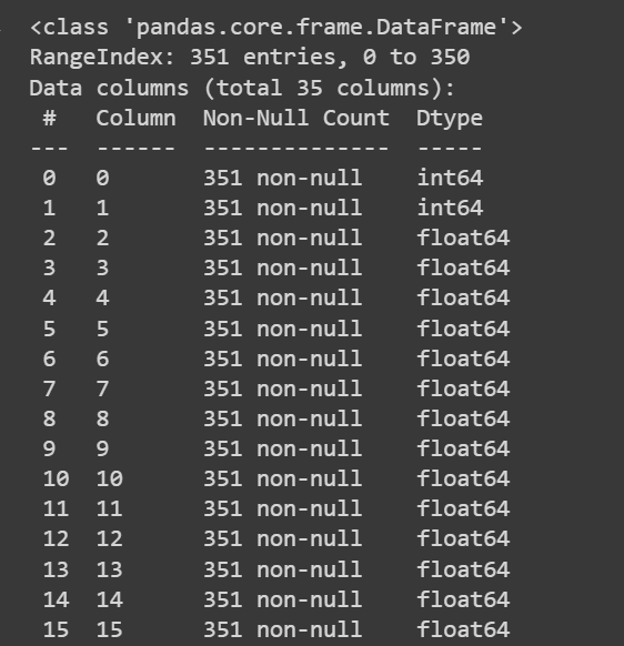 Truncated Output of df.information()
As a result of we’ve all numeric options, we will additionally get some descriptive statistics utilizing the describe() methodology on the dataframe:
# Get descriptive statistics of the dataset
print(df.describe())
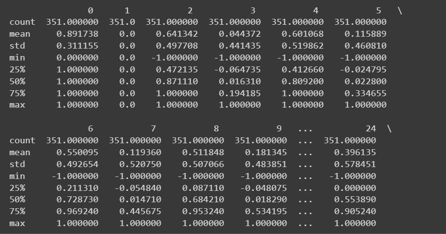
Truncated Output of df.describe()
The column names are at the moment 0 by means of 34—together with the label. As a result of the dataset doesn’t present descriptive names for the columns, it simply refers to them as attribute_1 to attribute_34 if you want you may rename the columns of the information body as proven:
column_names = [
"attribute_1", "attribute_2", "attribute_3", "attribute_4", "attribute_5",
"attribute_6", "attribute_7", "attribute_8", "attribute_9", "attribute_10",
"attribute_11", "attribute_12", "attribute_13", "attribute_14", "attribute_15",
"attribute_16", "attribute_17", "attribute_18", "attribute_19", "attribute_20",
"attribute_21", "attribute_22", "attribute_23", "attribute_24", "attribute_25",
"attribute_26", "attribute_27", "attribute_28", "attribute_29", "attribute_30",
"attribute_31", "attribute_32", "attribute_33", "attribute_34", "class_label"
]
df.columns = column_names
Observe: This step is only optionally available. You may proceed with the default column names for those who want.
# Show the primary few rows of the DataFrame
df.head()
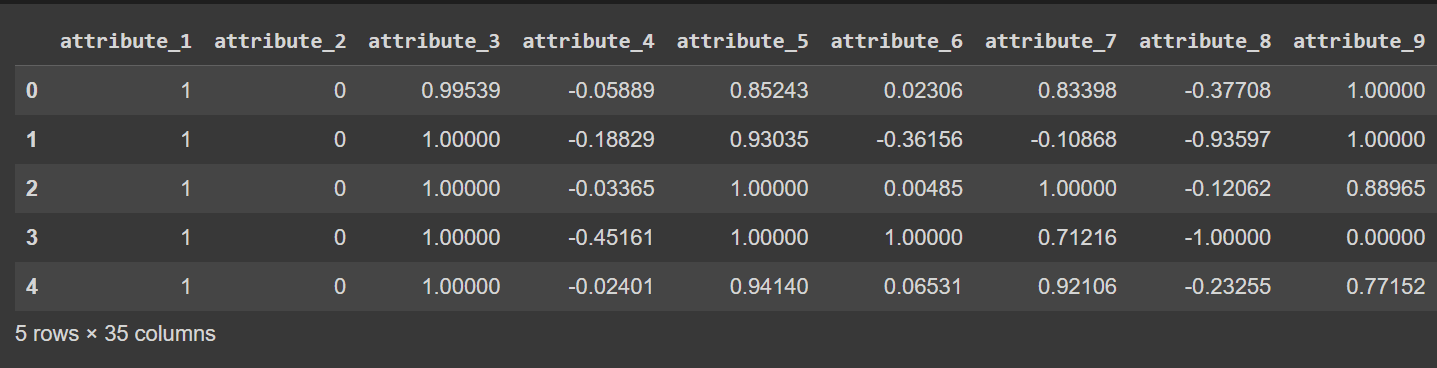
Truncated Output of df.head() [After Renaming Columns]
Step 3 – Renaming Class Labels and Visualizing Class Distribution
As a result of the output class labels are ‘g’ and ‘b’, we have to map them to 1 and 0 , respectively. You are able to do it utilizing map() or exchange():
# Convert the class labels from 'g' and 'b' to 1 and 0, respectively
df["class_label"] = df["class_label"].exchange({'g': 1, 'b': 0})
Let’s additionally visualize the distribution of the category labels:
import matplotlib.pyplot as plt

# Rely the variety of knowledge factors in every class
class_counts = df['class_label'].value_counts()

# Create a bar plot to visualise the category distribution
plt.bar(class_counts.index, class_counts.values)
plt.xlabel('Class Label')
plt.ylabel('Rely')
plt.xticks(class_counts.index)
plt.title('Class Distribution')
plt.present()
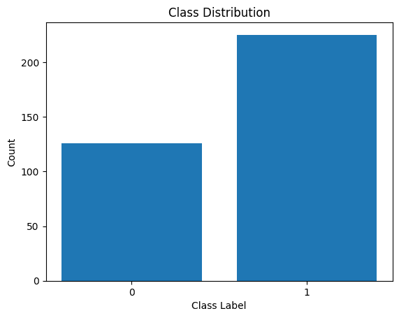
Distribution of Class Labels
We see that there’s an imbalance within the distribution. There are extra information belonging to class 1 than to class 0. We’ll deal with this class imbalance when constructing the logistic regression mannequin.
Step 5 – Preprocessing the Dataset
Let’s acquire the options and output labels like so:
X = df.drop('class_label', axis=1)  # Enter options
y = df['class_label']               # Goal variable
After splitting the dataset into the prepare and take a look at units, we have to preprocess the dataset.
When there are various numeric options—every on a probably completely different scale—we have to preprocess the numeric options. A typical methodology is to remodel them such that they observe a distribution with zero imply and unit variance.
The StandardScaler from scikit-learn’s preprocessing module helps us obtain this.
from sklearn.preprocessing import StandardScaler
from sklearn.model_selection import train_test_split

# Break up the dataset into coaching and testing units
X_train, X_test, y_train, y_test = train_test_split(X, y, test_size=0.2, random_state=42)

# Get the indices of the numerical options
numerical_feature_indices = record(vary(34))  # Assuming the numerical options are in columns 0 to 33

# Initialize the StandardScaler
scaler = StandardScaler()

# Normalize the numerical options within the coaching set
X_train.iloc[:, numerical_feature_indices] = scaler.fit_transform(X_train.iloc[:, numerical_feature_indices])

# Normalize the numerical options within the take a look at set utilizing the educated scaler from the coaching set
X_test.iloc[:, numerical_feature_indices] = scaler.remodel(X_test.iloc[:, numerical_feature_indices])
Step 6 – Constructing a Logistic Regression Mannequin
Now we will instantiate a logistic regression classifier. The LogisticRegression class is a part of scikit-learn’s linear_model module.
Discover that we’ve set the class_weight parameter to ‘balanced’. This may assist us account for the category imbalance. By assigning weights to every class—inversely proportional to the variety of information within the lessons.
After instantiating the category, we will match the mannequin to the coaching dataset:
from sklearn.linear_model import LogisticRegression

mannequin = LogisticRegression(class_weight="balanced")
mannequin.match(X_train, y_train)
Step 7 – Evaluating the Logistic Regression Mannequin
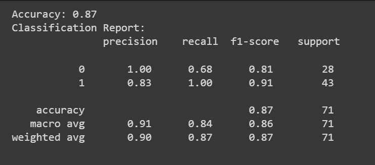
You may name the predict() methodology to get the mannequin’s predictions.
Along with the accuracy rating, we will additionally get a classification report with metrics like precision, recall, and F1-score.
from sklearn.metrics import accuracy_score, classification_report

y_pred = mannequin.predict(X_test)
accuracy = accuracy_score(y_test, y_pred)
print(f"Accuracy: {accuracy:.2f}")

classification_rep = classification_report(y_test, y_pred)
print("Classification Report:n", classification_rep)
Congratulations, you could have coded your first logistic regression mannequin!
On this tutorial, we realized about logistic regression intimately: from concept and math to coding a logistic regression classifier.
As a subsequent step, attempt constructing a logistic regression mannequin for an appropriate dataset of your alternative.
The Ionosphere dataset is licensed below a Artistic Commons Attribution 4.0 Worldwide (CC BY 4.0) license:
Sigillito,V., Wing,S., Hutton,L., and Baker,Okay.. (1989). Ionosphere. UCI Machine Studying Repository. https://doi.org/10.24432/C5W01B.
Bala Priya C is a developer and technical author from India. She likes working on the intersection of math, programming, knowledge science, and content material creation. Her areas of curiosity and experience embody DevOps, knowledge science, and pure language processing. She enjoys studying, writing, coding, and low! At the moment, she’s engaged on studying and sharing her information with the developer group by authoring tutorials, how-to guides, opinion items, and extra.