
Time collection evaluation is broadly used for forecasting and predicting future factors in a time collection. AutoRegressive Built-in Shifting Common (ARIMA) fashions are broadly used for time collection forecasting and are thought of one of the common approaches. On this tutorial, we are going to discover ways to construct and consider ARIMA fashions for time collection forecasting in Python.
The ARIMA mannequin is a statistical mannequin utilized for analyzing and predicting time collection knowledge. The ARIMA method explicitly caters to straightforward buildings present in time collection, offering a easy but highly effective technique for making skillful time collection forecasts.
ARIMA stands for AutoRegressive Built-in Shifting Common. It combines three key elements:
- Autoregression (AR): A mannequin that makes use of the correlation between the present statement and lagged observations. The variety of lagged observations is known as the lag order or p.
- Built-in (I): The usage of differencing of uncooked observations to make the time collection stationary. The variety of differencing operations is known as d.
- Shifting Common (MA): A mannequin takes under consideration the connection between the present statement and the residual errors from a shifting common mannequin utilized to previous observations. The dimensions of the shifting common window is the order or q.
The ARIMA mannequin is outlined with the notation ARIMA(p,d,q) the place p, d, and q are substituted with integer values to specify the precise mannequin getting used.
Key assumptions when adopting an ARIMA mannequin:
- The time collection was generated from an underlying ARIMA course of.
- The parameters p, d, q have to be appropriately specified primarily based on the uncooked observations.
- The time collection knowledge have to be made stationary through differencing earlier than becoming the ARIMA mannequin.
- The residuals needs to be uncorrelated and usually distributed if the mannequin matches nicely.
In abstract, the ARIMA mannequin offers a structured and configurable method for modeling time collection knowledge for functions like forecasting. Subsequent we are going to take a look at becoming ARIMA fashions in Python.
On this tutorial, we are going to use Netflix Inventory Knowledge from Kaggle to forecast the Netflix inventory worth utilizing the ARIMA mannequin.
Knowledge Loading
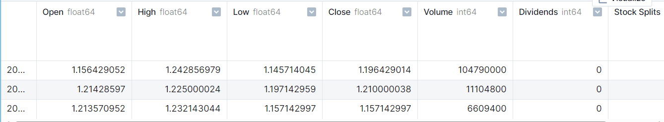
We’ll load our inventory worth dataset with the “Date” column as index.
import pandas as pd


net_df = pd.read_csv("Netflix_stock_history.csv", index_col="Date", parse_dates=True)
net_df.head(3)
Knowledge Visualization
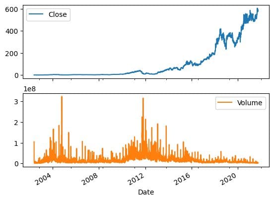
We will use pandas ‘plot’ operate to visualise the adjustments in inventory worth and quantity over time. It is clear that the inventory costs are rising exponentially.
net_df[["Close","Volume"]].plot(subplots=True, structure=(2,1));
Rolling Forecast ARIMA Mannequin
Our dataset has been cut up into coaching and take a look at units, and we proceeded to coach an ARIMA mannequin. The primary prediction was then forecasted.
We acquired a poor consequence with the generic ARIMA mannequin, because it produced a flat line. Subsequently, we have now determined to attempt a rolling forecast technique.
Be aware: The code instance is a modified model of the pocket book by BOGDAN IVANYUK.
from statsmodels.tsa.arima.mannequin import ARIMA
from sklearn.metrics import mean_squared_error, mean_absolute_error
import math


train_data, test_data = net_df[0:int(len(net_df)*0.9)], net_df[int(len(net_df)*0.9):]


train_arima = train_data['Open']
test_arima = test_data['Open']


historical past = [x for x in train_arima]
y = test_arima
# make first prediction
predictions = listing()
mannequin = ARIMA(historical past, order=(1,1,0))
model_fit = mannequin.match()
yhat = model_fit.forecast()[0]
predictions.append(yhat)
historical past.append(y[0])
When coping with time collection knowledge, a rolling forecast is usually obligatory as a result of dependence on prior observations. A technique to do that is to re-create the mannequin after every new statement is acquired.
To maintain observe of all observations, we are able to manually preserve an inventory referred to as historical past, which initially comprises coaching knowledge and to which new observations are appended every iteration. This method might help us get an correct forecasting mannequin.
# rolling forecasts
for i in vary(1, len(y)):
    # predict
    mannequin = ARIMA(historical past, order=(1,1,0))
    model_fit = mannequin.match()
    yhat = model_fit.forecast()[0]
    # invert reworked prediction
    predictions.append(yhat)
    # statement
    obs = y[i]
    historical past.append(obs)
Mannequin Analysis
Our rolling forecast ARIMA mannequin confirmed a 100% enchancment over easy implementation, yielding spectacular outcomes.
# report efficiency
mse = mean_squared_error(y, predictions)
print('MSE: '+str(mse))
mae = mean_absolute_error(y, predictions)
print('MAE: '+str(mae))
rmse = math.sqrt(mean_squared_error(y, predictions))
print('RMSE: '+str(rmse))
MSE: 116.89611817706545
MAE: 7.690948135967959
RMSE: 10.811850821069696
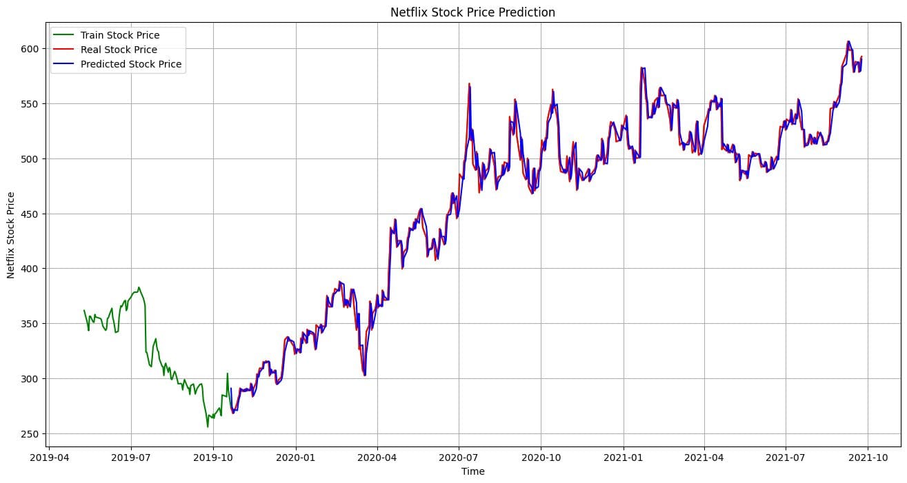
Let’s visualize and examine the precise outcomes to the expected ones . It is clear that our mannequin has made extremely correct predictions.
import matplotlib.pyplot as plt
plt.determine(figsize=(16,8))
plt.plot(net_df.index[-600:], net_df['Open'].tail(600), colour="inexperienced", label="Prepare Inventory Worth")
plt.plot(test_data.index, y, colour="crimson", label="Actual Inventory Worth")
plt.plot(test_data.index, predictions, colour="blue", label="Predicted Inventory Worth")
plt.title('Netflix Inventory Worth Prediction')
plt.xlabel('Time')
plt.ylabel('Netflix Inventory Worth')
plt.legend()
plt.grid(True)
plt.savefig('arima_model.pdf')
plt.present()
On this brief tutorial, we offered an summary of ARIMA fashions and how one can implement them in Python for time collection forecasting. The ARIMA method offers a versatile and structured method to mannequin time collection knowledge that depends on prior observations in addition to previous prediction errors. In the event you’re keen on a complete evaluation of the ARIMA mannequin and Time Collection evaluation, I like to recommend having a look at Inventory Market Forecasting Utilizing Time Collection Evaluation.
Abid Ali Awan (@1abidaliawan) is an authorized knowledge scientist skilled who loves constructing machine studying fashions. Presently, he’s specializing in content material creation and writing technical blogs on machine studying and knowledge science applied sciences. Abid holds a Grasp’s diploma in Know-how Administration and a bachelor’s diploma in Telecommunication Engineering. His imaginative and prescient is to construct an AI product utilizing a graph neural community for college kids fighting psychological sickness.